LR03: Residuals and RMSE
This is post #3 on the subject of linear regression, using R for computational demonstrations and examples. We cover here residuals (or prediction errors) and the RMSE of the prediction line. The first post in the series is LR01: Correlation.
- Acknowledgments: organization is extracted from:
- Freedman, Pisani, Purves, Statistics, 4th ed., probably the best book on statistical thinking (it maybe has a total of 4-5 formulas). It is referred here as FPP.
- A lot of what is good is due to Professor Rudy Guerra.
Previous
LR02: SD line, GoA, Regression
What we know so far
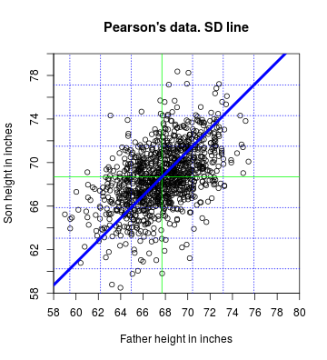
- Correlation coefficient: measure of linear association, or clustering about the SD line.
- If the scatterplot of both variables is a football-shaped cloud of points,
those points cluster about the SD line, and the relationship between both variables
can be summarized by:
- average of x-values, SD of x-values ($s_x$),
- average of y-values, SD of y-values ($s_y$).
-
the correlation coefficient r.
- Reminder: we are (still) not making any probabilistic assumption, so we are not treating any variable as random, so everything stays in lower case. We are only saying (for now) that the correlation coefficient makes sense, as a summary “descriptive” statistic, for football-shaped cloud of points (even non-random ones), and it makes progressively less sense the more we depart from a football-shaped cloud of points. Following this reasoning, we could be using standard deviation version FPP (dividing by $n$), or $s$ (dividing by $n-1$) because we are not using them to estimate $\sigma$ (the population standard deviation) as that would imply making probabilistic assumptions (by the way, both version of the standard deviations, even with the right probabilistic assumptions, are biased estimators of the population standard deviation).
- Graph of Averages (GoA): discrete function defined by $\text{Ave}(y|x)$, depending on the size of the $x$-intervals chosen (as happens with histograms):
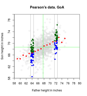
The GoA should always work, also for non football-shaped cloud of points.
-
The regression (or regression function), linear or non-linear, of $y$ (dependent variable) on $x$ (independent variable) is a continous function that is a “smoother” of the GoA (that is a “discrete” function). It always work (but we may not know its mathematical form). The regression is the continous version of $\text{Ave}(y|x)$ (GoA is the discrete version). If we are making probabilistic assumptions (by considering $Y$ a random variable with given characteristics that we will see later), we say that the regression function is the conditional expectaton of $Y$ given $X=x$ (or, in mathematical notation, $\text{E}(Y|X=x)$).
-
The regression line is a smoothed version of the GoA that is correct only when the GoA is linear.
-
When the GoA is linear, a best fit regression line, that passes through the point of averages $(\bar{x}, \bar{y})$, is found as:
where the slope $b$ is:
and the intercept $a$ is:
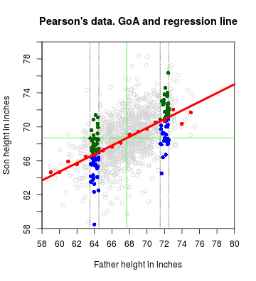
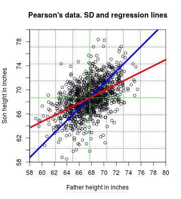
- The regression line is an attenuated version of the SD line (that has slope = $\frac{s_y}{s_x}$)
-
T or F: Regression is the line $y = a + bx$.
-
T or F: The SD line is the regression line.
Residuals, or Prediction errors
-
The regression method can be used to predict (guess) y from x (or x from y…). However, do you expect actual values to satisfy the predictions (guesses)?
-
They will differ, but, by how much? (What do you think?)
-
We will answer this in a little bit: we first need to consider the prediction errors, or residuals.
The distance of a point above (+) or below (-) the regression line is:
error = actual - predicted.
- In the Pearson’s data (which was the name of the red line plotted?), showing only distances for a subset of points, it looks like:
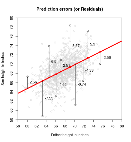
The prediction error is usually called residual. For consistency with Sheather’s book, we will name it $\hat{e}_i$ (you can also find it as $\hat{\epsilon}_i$, $r_i$, and perhaps other variants), the predicted value (or fitted value) is denoted by $\hat{y}_i$. The actual value is the y-coordinate of the point, $y_i$.
(Note: we are still not making any probabilistic assumptions, but hats are used to denote estimators, that are random variables. Even if usually random variables are denoted with upper case, residuals, or prediction errors, are usually denoted with lower case (the lower case also include errors $e_i$). When making probabilistic assumptions, $\hat{y}_i$ will become $\hat{Y}_i$. Sorry about the abuse of notation.)
Mathematically:
where
## Predicted points
yhat <- meany - r*sd(y)/sd(x)*meanx + r*sd(y)/sd(x)*x

## Prediction errors (residuals): actual - predicted
ehat <- y - yhat

hist(ehat, breaks = "Scott", probability = TRUE)
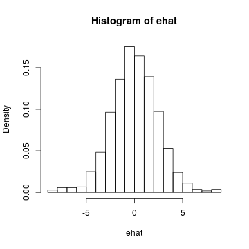
- The smaller the distance of each point to the line, the better the fit to the regression line.
The RMSE of the prediction line
RMSE stands for Root Mean Square Error. This implies:
- squaring the errors, or residuals:
- Finding their mean:
- Taking square root of the resulting mean:
Using R:
(RMSE <- sqrt(mean(ehat^2)))
## [1] 2.434294
- According to FPP, “the root mean square error for regression says how far typical points are above or below the regression line. The RMSE is to the regression line as the SD is to the average. For instance, if the scatter diagram is football-shaped, about 68% of the points on the scatter diagram will be within one RMSE of the regression line, about 95% of then will be within 2 RMSE of the regression line”.
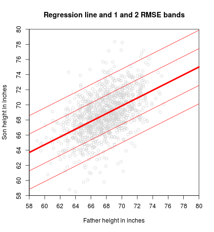
## Proportion of values contained between 1 RMSE
print(mean(abs(ehat) < RMSE))
## [1] 0.7133581
## Proportion of values contained between 2 RMSEs
print(mean(abs(ehat) < 2 * RMSE))
## [1] 0.9573284
-
Pretty good, no?
-
FPP also present a relation between RMSE and SDy (the one calculated by dividing by $n$)
Let’s get it with R:
## FPP version of sample standard deviation
SD <- function(x) sqrt(mean((x-mean(x))^2))

(RMSE2 <- sqrt(1-r^2)*SD(y))
## [1] 2.434294
RMSE
## [1] 2.434294
- The interpretation of RMSE is that it represents the typical size of the residuals.
Baby steps towards probabilistic assumptions
- When the cloud of points is football-shaped the distribution of $y$-values inside a strip is Normal with mean approximately equal to $\text{Ave}(Y|X=x)$ and standard deviation approximately equal to RMSE.
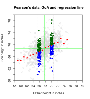
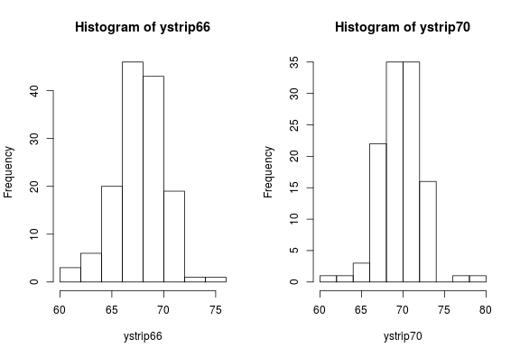
mean(ystrip66)
## [1] 67.65625
sd(ystrip66)
## [1] 2.350964
mean(ystrip70)
## [1] 69.76845
sd(ystrip70)
## [1] 2.48953
-
If we only know about $y$, and not $x$, what do we use as an approximation to the spread (variation) of $y$?
-
If we also know about $x$, what do we use as an approximation to the spread of $y$ in a strip?
-
How is RMSE in relation to SDy? (smaller, equal, bigger)?
In the case of sample data, as happened with SD, RMSE is not used nowadays because it is biased if used as an estimator of the standard deviation $\sigma$ of the residuals $e_i$ of the population (at some point we will calculate which is the bias of its square as an estimator of the variance $\sigma^2$ of $e_i$). Of course, this has importance only when we are dealing with samples and making probabilistic assumptions.
The version that is used, called Residual standard error, is also a biased estimator of $\sigma$, but its square (called Mean Square Error of the residuals and indicated by $\text{MS}_\text{res}$), is an unbiased estimator of the variance $\sigma^2$ of $e_i$.
To start getting used to the functions lm, summary and anova that we will use heavily for simple and multiple regression (we will learn more about them some posts from now), let’s see
where these values can be found.
fit <- lm(y ~ x)
(sfit <- summary(fit))
##
## Call:
## lm(formula = y ~ x)
##
## Residuals:
##     Min      1Q  Median      3Q     Max
## -8.8772 -1.5144 -0.0079  1.6285  8.9685
##
## Coefficients:
##             Estimate Std. Error t value Pr(>|t|)
## (Intercept) 33.88660    1.83235   18.49   <2e-16 ***
## x            0.51409    0.02705   19.01   <2e-16 ***
## ---
## Signif. codes:  0 '***' 0.001 '**' 0.01 '*' 0.05 '.' 0.1 ' ' 1
##
## Residual standard error: 2.437 on 1076 degrees of freedom
## Multiple R-squared:  0.2513,	Adjusted R-squared:  0.2506
## F-statistic: 361.2 on 1 and 1076 DF,  p-value: < 2.2e-16
The Residual standard error is easily spotted at the beginning of the third line starting from the bottom. It is rounded to three decimals. The actual value with more decimals (still rounded) is:
sfit$sigma
## [1] 2.436556
that is slightly different than:
RMSE
## [1] 2.434294
- How to “correct” RMSE to agree with Residual standard error?
RMSE * sqrt(n/(n - 2))
## [1] 2.436556
-
Now we are in peace. But… why $n - 2$ ???
-
We said that the Residual standard error is a (biased) estimator of $\sigma$. Its square, $\text{MS}_\text{res}$, is an unbiased estimator of $\sigma^2$.
sfit$sigma^2
## [1] 5.936804
Its value, using anova:
(afit <- anova(fit))
## Analysis of Variance Table
##
## Response: y
##             Df Sum Sq Mean Sq F value    Pr(>F)
## x            1 2144.6 2144.58  361.23 < 2.2e-16 ***
## Residuals 1076 6388.0    5.94
## ---
## Signif. codes:  0 '***' 0.001 '**' 0.01 '*' 0.05 '.' 0.1 ' ' 1
is found on the intersection of the row Residuals and the column Mean Sq. The less-rounded value is:
afit$"Mean Sq"[2]
## [1] 5.936804
Appendix
Code to load data and initial calculations
library(UsingR)

## Pearson's data
## Father and son data
data(father.son)

x <- father.son$fheight
y <- father.son$sheight

n <- length(x)

## Summary statistics
meanx <- mean(x)
meany <- mean(y)
r <- cor(x, y)
Code to produce the SD line plot
plot(x, y,
     xlim = c(58, 80), ylim = c(58, 80),
     xaxt = "n", yaxt = "n", xaxs = "i", yaxs = "i",
     main = "Pearson's data. SD line",
     xlab = "Father height in inches", ylab = "Son height in inches")
axp <- seq(58, 80, by = 2)
axis(1, at = axp, labels = axp)
axis(2, at = axp, labels = axp)

## Spread of the cloud
abline(v=meanx+c(-1,1)*sd(x), col="blue", lty=3)
abline(h=meany+c(-1,1)*sd(y), col="blue", lty=3)
abline(v=meanx+c(-2,2)*sd(x), col="blue", lty=3)
abline(h=meany+c(-2,2)*sd(y), col="blue", lty=3)
abline(v=meanx+c(-3,3)*sd(x), col="blue", lty=3)
abline(h=meany+c(-3,3)*sd(y), col="blue", lty=3)

## Point of averages (center of the cloud)
abline(v=meanx, col="green")
abline(h=meany, col="green")

## SD line using equation and sd
abline(a = meany - sd(y)/sd(x)*meanx,
       b = sd(y)/sd(x), col = "blue", lwd = 4)
Code to produce the Graph of averages plot
plot(x, y,
     xlim = c(58, 80), ylim = c(58, 80), col="lightgrey",
     xaxt = "n", yaxt = "n", xaxs = "i", yaxs = "i",
     main = "Pearson's data. GoA",
     xlab = "Father height in inches", ylab = "Son height in inches")
axp <- seq(58, 80, by = 2)
axis(1, at = axp, labels = axp)
axis(2, at = axp, labels = axp)

## Point of averages (center of the cloud)
abline(v=meanx, col="green")
abline(h=meany, col="green")

fround <- 72
abline(v=fround+c(-.5,.5), lty=3)
with(subset(father.son, round(fheight,0) == fround),
     points(fheight, sheight,
            pch=16, col=ifelse(sheight > meany + (fheight-meanx)/sd(x)*sd(y)*r, "darkgreen", "blue")))

fround <- 64
abline(v=fround+c(-.5,.5), lty=3)
with(subset(father.son, round(fheight,0) == fround),
     points(fheight, sheight,
            pch=16, col=ifelse(sheight > meany + (fheight-meanx)/sd(x)*sd(y)*r, "darkgreen", "blue")))

## Graph of averages.
sgav <- with(father.son, tapply(sheight, round(fheight,0), mean))
## sgavnum <- with(father.son, tapply(sheight, round(fheight,0), length))
points(as.numeric(names(sgav)), sgav, col="red", pch=16)
## text(as.numeric(names(sgav)), sgav, sgavnum, pos=3)
Code to produce the Graph of averages + regression line plot
plot(x, y,
     xlim = c(58, 80), ylim = c(58, 80), col="lightgrey",
     xaxt = "n", yaxt = "n", xaxs = "i", yaxs = "i",
     main = "Pearson's data. GoA and regression line",
     xlab = "Father height in inches", ylab = "Son height in inches")
axp <- seq(58, 80, by = 2)
axis(1, at = axp, labels = axp)
axis(2, at = axp, labels = axp)

## Point of averages (center of the cloud)
abline(v=meanx, col="green")
abline(h=meany, col="green")

fround <- 72
abline(v=fround+c(-.5,.5), lty=3)
with(subset(father.son, round(fheight,0) == fround),
     points(fheight, sheight,
            pch=16, col=ifelse(sheight > meany + (fheight-meanx)/sd(x)*sd(y)*r, "darkgreen", "blue")))

fround <- 64
abline(v=fround+c(-.5,.5), lty=3)
with(subset(father.son, round(fheight,0) == fround),
     points(fheight, sheight,
            pch=16, col=ifelse(sheight > meany + (fheight-meanx)/sd(x)*sd(y)*r, "darkgreen", "blue")))

## Graph of averages.
sgav <- with(father.son, tapply(sheight, round(fheight,0), mean))
## sgavnum <- with(father.son, tapply(sheight, round(fheight,0), length))
points(as.numeric(names(sgav)), sgav, col="red", pch=16)
## text(as.numeric(names(sgav)), sgav, sgavnum, pos=3)

## Regression line
abline(a=meany-r*sd(y)/sd(x)*meanx, b=r*sd(y)/sd(x), lwd=4, col="red")
Code to produce the Residual plot
plot(x, y,
     xlim = c(58, 80), ylim = c(58, 80), col = "lightgrey",
     xaxt = "n", yaxt = "n", xaxs = "i", yaxs = "i",
     main = "Prediction errors (or Residuals)",
     xlab = "Father height in inches", ylab = "Son height in inches")
axp <- seq(58, 80, by = 2)
axis(1, at = axp, labels = axp)
axis(2, at = axp, labels = axp)

## Regression line
abline(a = meany - r*sd(y)/sd(x)*meanx, b = r*sd(y)/sd(x), lwd = 4, col = "red")

## for (fn in sample(nrow(father.son), 20)) {
for (i in c(39, 158, 204, 479, 686, 808, 844, 851, 852, 1070)) {
  ## Actual point
  points(x[i], y[i])
  ## Predicted point yhat_i
  yhat_i <- r*sd(y)/sd(x)*x[i] + meany-r*sd(y)/sd(x)*meanx
  points(x[i], yhat_i, pch=16, col="red")

  lines(rep(x[i], 2), c(y[i], yhat_i))

  ## Prediction error (or residual): actual - predicted
  ehat_i <- y[i] - yhat_i

  text(x[i], (y[i] + yhat_i)/2, round(ehat_i, 2), pos = 4)
}
Code to produce the histogram of the residuals
## Predicted points
yhat <- meany - r*sd(y)/sd(x)*meanx + r*sd(y)/sd(x)*x

## Prediction errors (residuals): actual - predicted
ehat <- y - yhat

hist(ehat, breaks = "Scott", probability = TRUE)
Code to produce the RMSE bands
## RMS error for regression

plot(x, y,
     xlim = c(58, 80), ylim = c(58, 80), col = "lightgrey",
     xaxt = "n", yaxt = "n", xaxs = "i", yaxs = "i",
     main = "Regression line and 1 and 2 RMSE bands",
     xlab = "Father height in inches", ylab = "Son height in inches")
axp <- seq(58, 80, by = 2)
axis(1, at = axp, labels = axp)
axis(2, at = axp, labels = axp)

## Regression line
a <- meany - r*sd(y)/sd(x)*meanx
b <- r*sd(y)/sd(x)

abline(a = a, b = b, lwd = 4, col = "red")

abline(a = a - 2 * RMSE, b = b, lwd = 1, col = "red")
abline(a = a - 1 * RMSE, b = b, lwd = 1, col = "red")
abline(a = a + 1 * RMSE, b = b, lwd = 1, col = "red")
abline(a = a + 2 * RMSE, b = b, lwd = 1, col = "red")
Code to produce the Graph of averages with strips of points
plot(x, y,
     xlim = c(58, 80), ylim = c(58, 80), col="lightgrey",
     xaxt = "n", yaxt = "n", xaxs = "i", yaxs = "i",
     main = "Pearson's data. GoA and regression line",
     xlab = "Father height in inches", ylab = "Son height in inches")
axp <- seq(58, 80, by = 2)
axis(1, at = axp, labels = axp)
axis(2, at = axp, labels = axp)

## Point of averages (center of the cloud)
abline(v=meanx, col="green")
abline(h=meany, col="green")

fround <- 66
abline(v=fround+c(-.5,.5), lty=3)
with(subset(father.son, round(fheight,0) == fround),
     points(fheight, sheight,
            pch=16, col=ifelse(sheight > meany + (fheight-meanx)/sd(x)*sd(y)*r, "darkgreen", "blue")))

fround <- 70
abline(v=fround+c(-.5,.5), lty=3)
with(subset(father.son, round(fheight,0) == fround),
     points(fheight, sheight,
            pch=16, col=ifelse(sheight > meany + (fheight-meanx)/sd(x)*sd(y)*r, "darkgreen", "blue")))

## Graph of averages.
sgav <- with(father.son, tapply(sheight, round(fheight,0), mean))
## sgavnum <- with(father.son, tapply(sheight, round(fheight,0), length))
points(as.numeric(names(sgav)), sgav, col="red", pch=16)
## text(as.numeric(names(sgav)), sgav, sgavnum, pos=3)
Code to produce the histograms of the strips
par(mfrow=c(1,2))

fround <- 66
ystrip66 <- with(subset(father.son, round(fheight,0) == fround),
                 sheight)
hist(ystrip66, breaks = 7)

fround <- 70
ystrip70 <- with(subset(father.son, round(fheight,0) == fround),
                 sheight)
hist(ystrip70, breaks = 7)
Previous
LR02: SD line, GoA, Regression